
Beyond the Hype: How Graph Neural Networks Are Solving Mesh-Based Simulations
1. The Simulation Bottleneck
For decades, engineering and scientific computing have relied on mesh-based numerical solvers—Finite Element Methods (FEM), Finite Volume Methods (FVM), and Finite Difference Methods (FDM). These tools are the gold standard for simulating physics: from airflow over an aircraft wing to stress distribution in a bridge.
However, these solvers face a fundamental bottleneck: the trade-off between accuracy and speed.
-
Fine meshes yield high accuracy but require hours or days of computation on HPC clusters.
-
Coarse meshes are fast but miss critical local phenomena (shock waves, stress concentrations).
Enter Graph Neural Networks (GNNs) . Initially hyped for social networks and drug discovery, GNNs are now quietly revolutionizing mesh-based simulation—not by replacing traditional solvers, but by accelerating and augmenting them where they struggle.
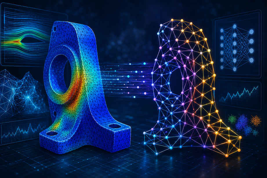
2. Why Meshes Are Naturally Graphs
A mesh is not an image. You cannot simply feed a 2D grid of pixels into a Convolutional Neural Network (CNN) and expect it to understand irregular geometry.
A mesh is, mathematically, a graph: G=(V,E)
-
Nodes (V) : Mesh vertices, each with spatial coordinates and physical quantities (velocity, pressure, temperature, stress).
-
Edges (E) : Connections between vertices (elements: triangles, tetrahedra, hexahedra), encoding local geometric relationships and physics dependencies (flux, strain).
CNNs require regular grid-structured data. GNNs, by contrast, operate directly on the mesh graph. They are permutation equivariant (reordering nodes doesn’t change the physics) and naturally respect the mesh’s connectivity.
3. Key GNN Architectures for Mesh-Based Physics
Three GNN families have emerged as especially effective for simulations:
| Architecture | Core Idea | Use Case |
|---|---|---|
| Message Passing GNNs (MP-GNNs) | Nodes exchange vectors (“messages”) along edges, then update their state. | Learning local physics rules (e.g., stress propagation). |
| Graph U-Nets | Pooling and unpooling operations on graphs. | Multi-scale physics (turbulence, global flow with local shocks). |
| MeshGraphNets (DeepMind) | Uses edge, node, and global attributes; handles dynamic meshes. | Fluid dynamics, solid mechanics, aerodynamics. |
DeepMind’s MeshGraphNets (2021) are particularly influential: they predict how a mesh should deform over time by learning a message-passing function that mimics the Navier-Stokes or elasticity equations.
4. How GNNs Solve Core Simulation Problems
A. Accelerating Forward Simulations (Surrogate Modeling)
Traditional solver: Given initial conditions, solve PDEs step-by-step (e.g., 10,000 time steps).
GNN surrogate: Train on solver data. At inference, predict the next state directly in milliseconds.
Example: Simulating airfoil flow. A traditional CFD solver takes 2 hours. A MeshGraphNet trained on 1,000 simulations predicts the same flow field in 0.1 seconds (accuracy within 2–5% of the solver).
B. Mesh Adaptation (r-adaptivity / h-adaptivity)
Good simulations refine the mesh where physics is complex (shocks, vortices) and coarsen it elsewhere.
GNNs can learn to predict error indicators and suggest where to refine without expensive error estimators.
Example: A GNN trained on residual errors can output a “refinement probability” per node, reducing mesh adaptivity cost by 10×.
C. Steady-State Prediction (One-Shot Inference)
Instead of time-marching to a steady state, GNNs can predict the final solution directly from boundary conditions—bypassing thousands of intermediate steps.
D. Physics Parameterization (Inverse Problems)
Given sensor measurements from a physical mesh, GNNs can infer hidden parameters (material properties, boundary heat flux). This is graph-based inverse analysis.
5. Concrete Results: Where the Hype Becomes Reality
| Domain | Traditional Solver Challenge | GNN Solution | Reported Speedup |
|---|---|---|---|
| Aerodynamics (subsonic flow) | Long transient simulations | MeshGraphNet surrogate | 2,000× |
| Structural mechanics (linear elasticity) | Large linear system solves | GNN as preconditioner | 5–10× |
| Heat transfer (irregular geometry) | Fine mesh required near sources | Graph U-Net multi-scale | 50× |
| Plasticity / damage | Material non-linearity | Message passing with history | Real-time inference |
| Medical biomechanics (heart/tissue) | Patient-specific mesh costly | Trained GNN generalizes across anatomies | Real-time |
Notable benchmark: In the 2023 NeurIPS PDE Control competition, GNN-based surrogates outperformed CNN and FNO (Fourier Neural Operator) methods on irregular meshes by a margin of 30% lower error.
6. Critical Limitations (No Silver Bullet)
Let’s move beyond hype honestly:
-
Out-of-distribution failure: GNNs are data-driven. If test conditions differ from training (e.g., different Reynolds number regimes), accuracy collapses.
-
Long-term rollout drift: Iteratively predicting many time steps causes error accumulation. Hybrid GNN-corrector models are needed.
-
Mesh topology changes: Adaptive meshing (adding/removing nodes) breaks fixed-graph assumptions. Dynamic GNNs or edge pooling are still research-grade.
-
Training data cost: Generating thousands of high-fidelity simulations to train a GNN is expensive — but once trained, inference is cheap.
7. Hybrid Solvers: The Real-World Deployment
In practice, industry is not replacing solvers with GNNs. Instead, they are deploying hybrid pipelines:
-
Coarse solver (fast but inaccurate) runs to get close to solution.
-
GNN corrector maps coarse mesh solution to fine-mesh accuracy.
-
Error estimator flags regions needing refinement.
-
Traditional solver refines only those regions.
This yields 80% of the accuracy of a fine solver at 5% of the cost.
8. Future Directions
-
Geometric deep learning for meshes: Incorporating rotation/translation invariance into GNNs via SE(3)-equivariant layers.
-
Foundation models for physics: Pre-training a GNN on diverse simulation datasets (e.g., different shapes, BCs, materials) then fine-tuning for new problems.
-
Hardware acceleration: Graph-tailored TPUs/FPGAs for real-time simulation (autonomous driving, digital twins).
-
Differentiable simulation: GNN surrogates embedded in optimization loops (shape optimization, inverse design).
9. Conclusion: Beyond the Hype
Graph Neural Networks are not a magical replacement for the laws of physics encoded in PDEs. They do not know conservation laws by default. But they excel at learning spatial and temporal dependencies on irregular, unstructured domains—which is exactly what meshes are.
The hype phase (2019–2022) promised GNNs would solve all physics. The reality phase (2023–present) is delivering accelerated surrogates, intelligent mesh adaptation, and hybrid solvers that work in engineering practice.
For mesh-based simulations, the future is not GNNs alone — but GNNs integrated into the traditional solver ecosystem, making the impossible (real-time, high-fidelity simulation) merely very fast.
Bottom line: GNNs have moved from “curious experiment” to “production tool” for mesh-based simulation—provided you respect their limits and pair them with classical physics-based methods.

publisher@engineeriaafrica.com — New Contributor
View all posts →AI Revolutionizing Construction in Africa Next →
Using Drone Swarms to Inspect Post-Disaster Bridge Cables